Lorenz Attractor

Edward Lorenz was an American mathematician and pioneer of chaos theory. Lorenz built mathematical models of the motion of air in the atmosphere.

His original model involved a set of 12 nonlinear differential equations and discovered complex movements that were highly dependent upon the initial conditions of the system. He then looked for complex behaviour in simpler models. He built a simple model of a gas in a solid rectangular box with a heat source at the bottom.

The Lorenz attractor is a simplified model of convection of a gas within a confined space. This very simple model results in some very interesting motion, an example of deterministic chaos. A chaotic system is very sensitive to initial conditions and the system rapidly diverges.

The system is described by three coupled non-linear differential equations:

\begin{align} \frac{dx}{dt} & = a (y - x) \\ \frac{dy}{dt} & = x (b - z) - y \\ \frac{dz}{dt} & = xy - cz \\ \end{align}

where

a is the Prandtl number that represents the ratio of fluid viscosity to thermal conductivity
b is the Rayleigh number representing the difference in temperature between the top and bottom of the box
c is the ratio of the width to the height of the box

Commonly used constants are a = 10, b = 28 and c = 8/3.

In order to produce a POV-Ray render, we first need to set up a light source and a camera

light_source {
  0*x
  color rgb 1.0
  area_light
            <8, 0, 0> <0, 0, 8> 6, 4
  adaptive 3
  translate <0, 0, -10>
}
camera {	
	location <0, 20, -60>		           
	look_at <0,0,0>       
	rotate <0,0,0>
}

The equation above can be calculated in POV-Ray with

#local x1=x0+dT*a*(y0-x0);
#local y1=y0+dT*(x0*(b-z0)-y0);
#local z1=z0+dT*(x0*y0-c*z0);

We can wrap this in a macro to repeatedly calculate the points x, y and z over multiple iterations and draw spheres of radius R at each point.

#macro Lorenz(a, b, c, dT, Iter, x0, y0, z0, R)     
 #local Count=0;
 #while (Count < Iter) 
  #local x1=x0+dT*a*(y0-x0);
  #local y1=y0+dT*(x0*(b-z0)-y0);
  #local z1=z0+dT*(x0*y0-c*z0);
  sphere {
   <x1,y1,z1>, R
    pigment {
     rgb <0.9-(Count/Iter)*0.7,0.6,0.2+(Count/Iter)*0.7>
    }
    finish {
      diffuse 0.7
      ambient 0.9
      specular 0.3
      reflection {
       0.8  metallic
      }
    }
   }
  #local Count=Count+1;
  #local x0=x1;
  #local y0=y1;
  #local z0=z1;
 #end
#end

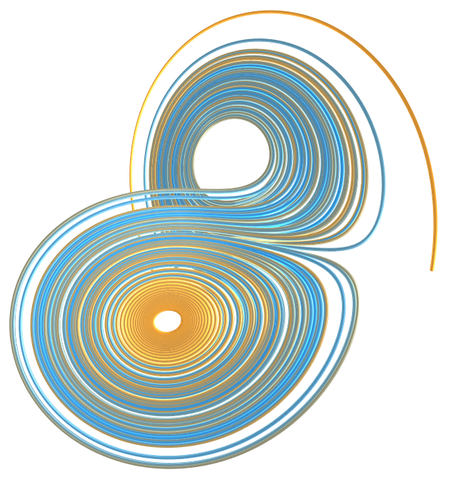
We colour the spheres based on their iteration, to make the whole thing look pretty. The image above is rendered with 40000 spheres, calling the macro with

Lorenz(10, 28, 8/3, 0.00022, 400000, 0.0001, 0.0001, 0.0001, 0.1)

In POV-Ray, we can produce animations by rendering frames with the clock variable and parameters set in an INI file

Antialias=On
Antialias_Threshold=0.1
Antialias_Depth=5
Input_File_Name=LorenzAttractor.pov
Initial_Frame=0
Final_Frame=5000
Initial_Clock=0
Final_Clock=1
Cyclic_Animation=on
Pause_when_Done=off

In our case, it is quite simple to produce a nice animation of building up the attractor as we just call the Lorenz macro with the iterations determined by the clock variable

Lorenz(10, 28, 8/3, 0.00022, 400000*clock, 0.0001, 0.0001, 0.0001, 0.1)

We can go one step further and draw a larger, red sphere at the final calculated value.

#macro LorenzPoint(a, b, c, dT, Iter, x0, y0, z0, R)
 #local Count=0;
 #while (Count<Iter) 
 #local x1=x0+dT*a*(y0-x0);
   #local y1=y0+dT*(x0*(b-z0)-y0);
   #local z1=z0+dT*(x0*y0-c*z0);
   #local Count=Count+1;
   #local x0=x1;
   #local y0=y1;
   #local z0=z1;
  #end
  sphere {
   <x1,y1,z1>, R
   pigment {
    rgb <0.9,0.3,0.3>
   }
   finish{
    diffuse 0.1
    ambient 0.99
    specular 0.3
    reflection {
      0.9  metallic
    }
  }
 }
#end

We can put in a sky sphere and a checkered plane, to add some depth to the render

plane { y, -25
  pigment { checker rgb <0.1, 0.1, 0.1> rgb <1.0, 1.0, 1.0> scale 5 }
  finish { reflection 0.2 ambient 0.4 }
	}
	fog {
  distance 100
  color rgb 0.9
  fog_offset 2
  fog_alt 5
  fog_type 2
}
sky_sphere {
  pigment { gradient y
  	color_map {
    [0 rgb <0.5, 0.6, 1> ]
    [1 rgb <0, 0, 1> ]
  	}
  }
  pigment { wrinkles turbulence 0.7
  	color_map {
    [0 rgbt <1,1,1,1>]
    [0.5 rgbt <0.98, 0.99, 0.99, .6>]
    [1 rgbt <1, 1, 1, 1>]
  	}
  	scale <.8, .1, .8>
  }
}

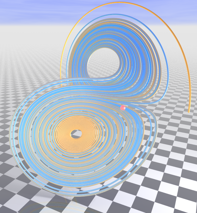
By rendering enough frames, we can produce a smooth animation building up the Lorenz attractor. The animation below is produced by 5000 frames, rendered over 3 days or so.

You can see the full code at the Github repository for this project.

Resources: