The Three-Scroll Unified Chaotic System (TSUCS) was introduced by Lin Pan, Wuneng Zhou, Jian’an Fang and Dequan Li in a paper submitted to the International Journal of Nonlinear Science in 2010. The TSUCS contains both a Lorenz-style attractor and also a Lu Chen-style attractor at its extremes.
\begin{align} \frac{dx}{dt} & = \textrm{a} (y - x) + \textrm{d} x y \\ \frac{dy}{dt} & = \textrm{c}x - xy + \textrm{f}y \\ \frac{dz}{dt} & = \textrm{b}z + yx - \textrm{e}x^2 \\ \end{align}
where I use the parameters\begin{align} \textrm{a} & = 40 \\ \textrm{b} & = 1.833 \\ \textrm{c} & = 55 \\ \textrm{d} & = 0.16 \\ \textrm{e} & = 0.65 \\ \textrm{f} & = 20 \end{align}
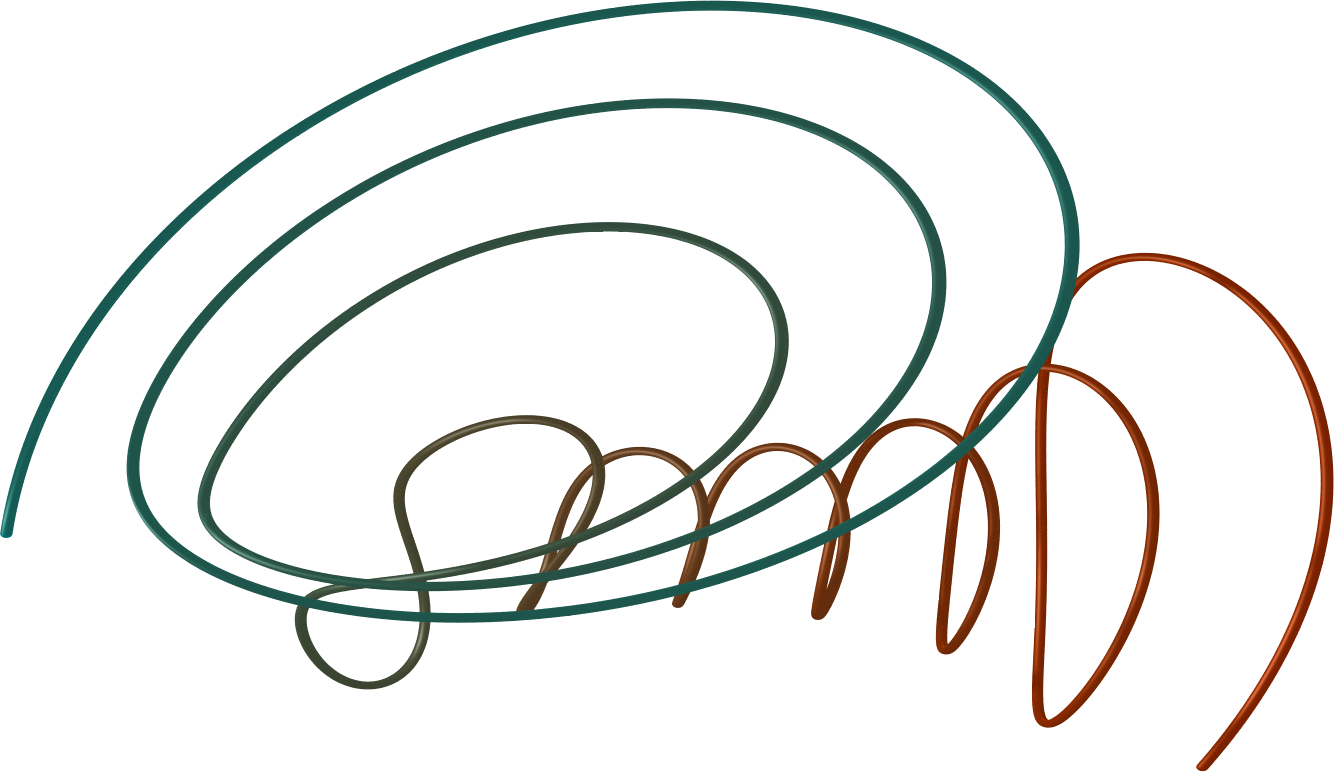
This attractor is quite beautiful as it starts off initially creating a corkscrew structure.
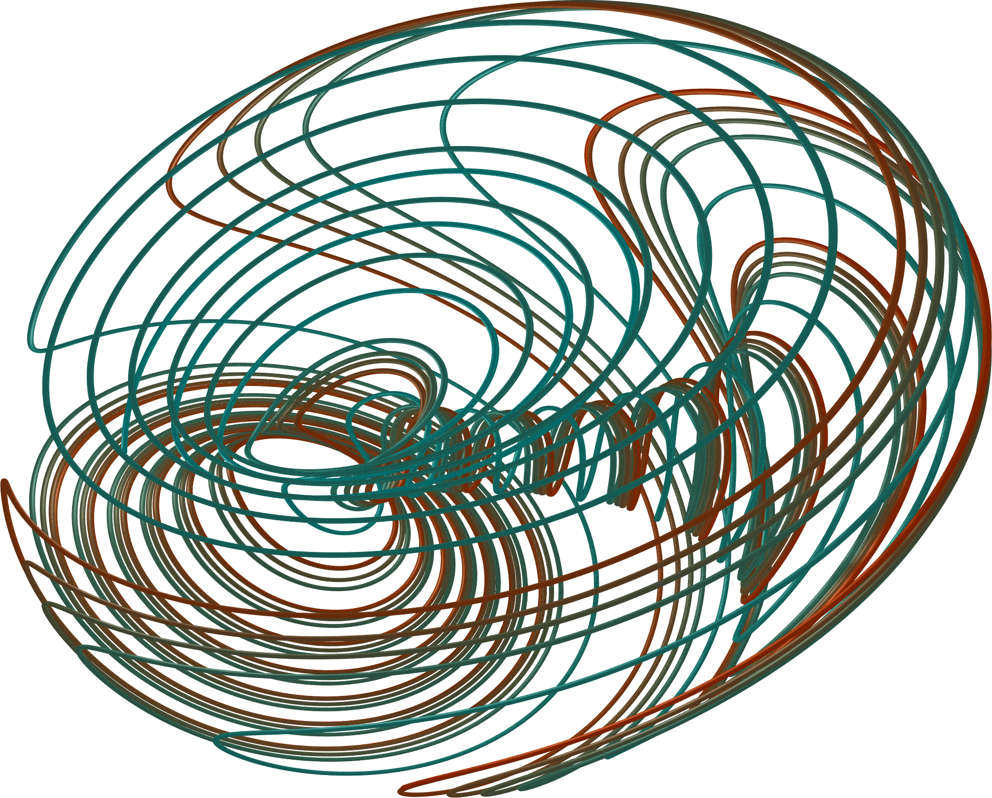
As it continues, it creates a spherical structure around it while retracing the previous structure.
The POV-Ray macro for rendering this attractor is:
#macro TSUCS(a, b, c, d, e, f, dT, Iter, x0, y0, z0, R)
    #local Count=0;
	#while (Count<Iter)
		#local x1=x0+dT*(a*(y0-x0) + (d*x0*z0));
		#local y1=y0+dT*((c * x0) - (x0*z0) + (f*y0));
        #local z1=z0+dT*((b * z0) + (x0 * y0) - (e * x0 * x0));
        #if(Count < (Iter - 1500))
    		sphere {
    		    <x1,y1,z1>, R
                pigment {
                    rgb <0.9-(Count/Iter)*0.7,0.6,0.2+(Count/Iter)*0.7>
                }
                finish {
                    diffuse 0.7
                    ambient 0.3
                    specular 0.5
                    reflection {
                        0.9  metallic
                    }
                }
            }
        #else
            sphere {
                <x1,y1,z1>, R
                pigment {
                    rgb <(Count/Iter),(Count/Iter)*0.25,(Count/Iter)*0.25>
                }
                finish{
                    diffuse 0.7
                    ambient 0.9
                    specular 0.3
                    reflection {
                        0.8  metallic
                    }
                }
            }
        #end
		#local Count=Count+1;
		#local x0=x1;
		#local y0=y1;
		#local z0=z1;
	#end
#end
This renders a series of spheres according to the differential equations. This also renders a red trace for the most recent points.
To run this macro we use, where the 'clock' variable controls the animation
TSUCS(40, 1.833, 55, 0.16,0.65,20,0.00002, 1000000*clock, 0.0001, 0.0001, 0.0001, 1)
We can also add a skysphere and checkered floor to make the scene look nice
light_source {
  0*x
  color rgb 1.0
  area_light
  <8, 0, 0> <0, 0, 8>
  6, 4
  adaptive 3
  translate <0, 0, -10>
}
camera {
	location <0, 20, -500>
	look_at <20-(50*clock),5,0>
	rotate <0,-90+(180*clock),0>
}
plane { y, -220
		pigment { checker rgb <0.1, 0.1, 0.1> rgb <1.0, 1.0, 1.0> scale 5 }
		finish { reflection 0.2 ambient 0.4 }
	}
	fog {
		distance 1000
		color rgb 0.9
		fog_offset 2
		fog_alt 5
		fog_type 2
	}
sky_sphere {
		pigment { gradient y
			color_map {
				[0 rgb <0.5, 0.6, 1> ]
				[1 rgb <0, 0, 1> ]
			}
		}
		pigment { wrinkles turbulence clock
			color_map {
				[0 rgbt <1,1,1,1>]
				[0.5 rgbt <0.98, 0.99, 0.99, .6>]
				[1 rgbt <1, 1, 1, 1>]
			}
			scale <.8, .1, .8>
		}
	}
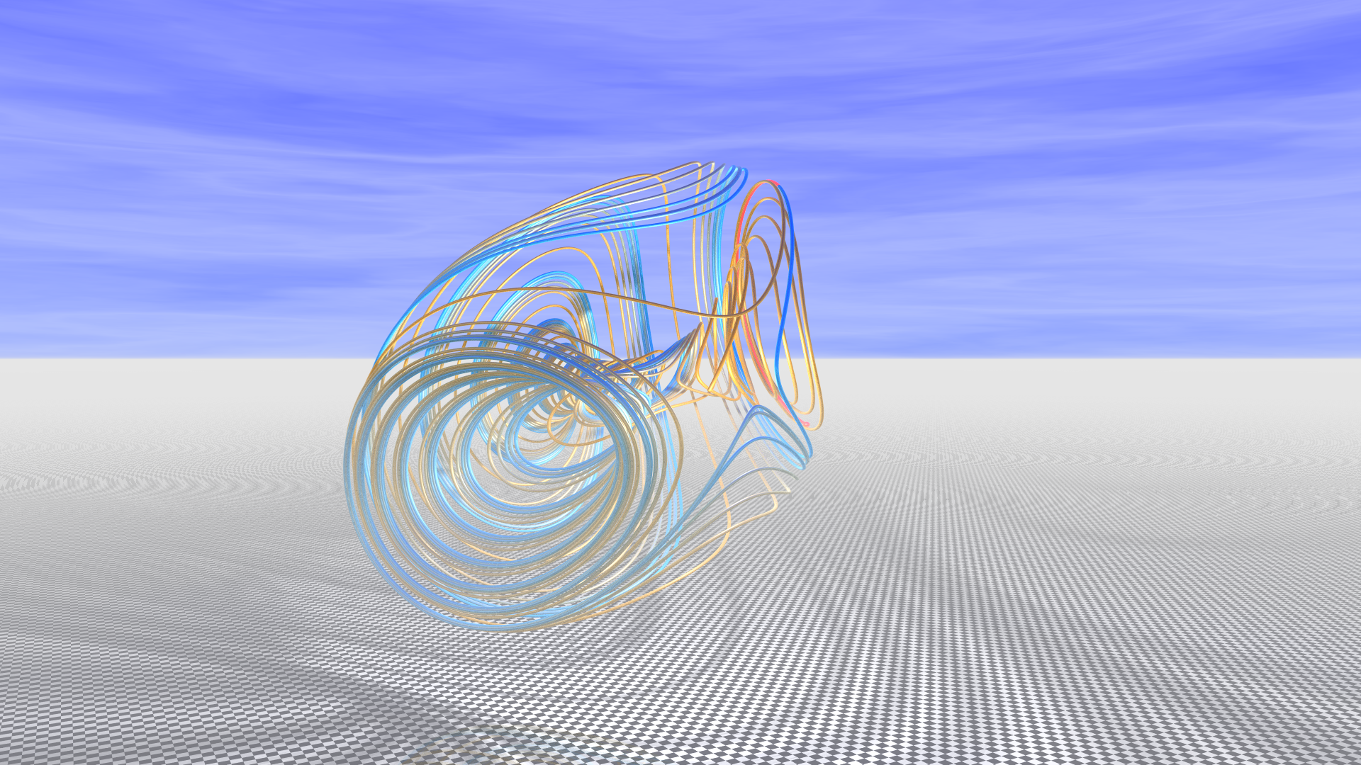
See below for a video of the render of this attractor building up